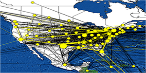
Simplified Systematic Network Planning – step 5

STEP 5: EVALUATE ALTERNATIVES
In Step 5, the planner evaluates the network plans developed in Step 4 by running several alternative scenarios.

Evaluation takes two forms:

• Cost analysis – comparing relevant costs among scenarios and their network plans.
• Intangible analysis – for factors or considerations that cannot be easily modeled or measured in economic terms.

0907_LIA_pg31_1

Cost analysis is generally straightforward.

Modeling software typically computes each alternative’s difference from the baseline on each element of total cost. But when comparing alternatives, planners must decide whether to show all costs or only those that are affected by the proposed alternatives.

In the MTT example, as shown in the Alternatives Analysis Worksheet, the four alternative plans compare what the company’s historical costs would have been if 32 oz capacity had been added in one of four existing plants.

Madison’s costs (Alt IV) are highest. Vicksburg’s costs (Alt III) are the lowest, and would have saved about $739,000 per year over the current or baseline network, and saved about $1 million more per year than Madison. These savings easily justify the upgrade of a production line.

Note that the planners have dropped purchasing costs from the previous Step 4 cost summary since these costs are unaffected and the same for all plans. This action helps to accentuate the cost differences between the alternatives. (See line 5 of the Cost Summary section in the Alternatives Analysis Worksheet.)

Naturally we would like to implement the network plan with the lowest total cost. But intangible factors or considerations may also play a role. For MTT, annual costs differ by only four percent among the four alternatives. With such a small difference, costs alone should not decide which plan is best. When two or more plans yield similar costs, the best one is typically found by comparing such intangibles as:

• Ease of implementation
• Exposure to various risks
• Fit with organization structure
• Labor-related considerations
• Facilities-related considerations

To evaluate intangibles, SSNP uses the weighted-factor approach shown in the lower portion of the Alternatives Analysis Worksheet. The planners list relevant factors and management assigns weights reflecting their relative importance. By convention, SSNP assigns a weight of 10 to the most important factor. Next, those who will implement and operate the network discuss and rate the effectiveness of each alternative on each factor. SSNP uses the vowel-code convention of A, E, I, O, U and X, in descending order of effectiveness, where A=4, E=3, I=2, O=1, and U=0. A rating of “X” disqualifies a plan unless the objectionable feature can be fixed.

After all plans have been rated on all factors, the ratings’ numerical values are multiplied by the factor weights to arrive at total scores for each plan. The highest score indicates the best network plan from an intangibles perspective. Hopefully the highest scoring plan will also have the lowest total cost. But if not, this procedure will reveal the intangible benefits of the more costly network plans. When cost comparison results in a stand-off and does not indicate a clear winner, the weighted factor approach will help discover which plan is best and why.

In the example, Alternative II (Briansville) scores roughly 50 percent (84/54) better than the lowest cost Alternative III, Vicksburg. Briansville offers more capacity relief, easier implementation, and a better fit with the current organizational structure. For these reasons, MTT management selected Briansville for the 32 oz bottling line upgrade.


Simplified Systematic Network Planning – step 4

STEP 4: CREATE SCENARIOS
In Step 4, the planner develops scenarios to model various elements of the problem. Each scenario is generated by making one or more of the following changes to the baseline model set-up:

• Adding or deleting products, locations, resources or lanes
• Changing demand allocations
• Adding or relaxing constraints.

0907_LIA_pg30

The Scenario Summary Sheet (overleaf) records these changes to the baseline model and the results of the scenario model runs. Changes and model results are summarized in terms of demand, resource utilization, lanes, and flow. A diagram visualizes the scenario network. In this way, each scenario represents an alternative network plan.

Often, those managing the network and its resources will be skeptical and reluctant to accept an initial scenario run that predicts significant cost savings from current conditions. These results may be characterized as “too optimistic”. The assumptions, parameters or constraints may be challenged and adjusted until the scenario run yields a more modest improvement – one that the line organization is willing to be accountable for obtaining.

But such a “pessimistic” outcome may be resisted by the planners who rightfully have faith in their validated model. The wise planner anticipates this give and take, and budgets time for optimistic, pessimistic, and most-likely cases. These can then be presented to management to show the likely range of scenario outcomes.

For MTT, several scenarios place the 32 oz upgrade at different plants. Each scenario was run with optimistic, pessimistic, and most-likely cases. Scenario I upgrades a production line in Jonesville (P1). Lanes to branch distribution centers are set up to receive products from Jonesville or Sommersville, with an added constraint that each DC order must be for a full truckload.

When the model was run, the optimizer moved 300,000 cases of 32 oz production from Sommersville to Jonesville. Of these cases, 200,000 were formerly cross-docked through Jonesville to its branch DCs. In terms of resources, Sommersville was relieved of 450 hours of production, while 300 hours were added to Jonesville. The difference is due to the greater efficiency of the newly upgraded line in Jonesville.

Simpsons (DC 23) could not satisfy the full truckload constraint from Jonesville and was reassigned to Sommersville. DCs 11 & 12 – Harrystown and Clinton, along with all the Virginia and West Virginia DCs, received all of their 32 oz products from Jonesville.

Often, some cost categories of concern at the outset of modeling prove to be insignificant once results are in. Or, an important stakeholder may have a fixation on some minor element of network cost. The Cost Summary section of the Scenario Summary Sheet includes these minor or occasionally irrelevant costs in order to remove any concerns or doubts. In our model, crossdocking costs and reduced overtime are insignificant and do not matter to the choice of network plan. Yet the planner includes these to satisfy the concerns and interests of key decision-makers.


Simplified Systematic Network Planning – step 3

STEP 3: ANALYZE SENSITIVITIES
In Step 3, the planner runs the model using optimization software; identifies any infeasibilities, and then troubleshoots.

Once free from infeasibilities, the planner runs and fine tunes the model, establishing a baseline that replicates current network performance.

0907_LIA_pg29

Model results for demand, costs and constraints are summarized on the Baseline Validation Worksheet. They are compared to the to the actual performance of the current network for the same time period. Notes and explanations address any changes made to the model and reasons for the variances between model results and actual performance. This exercise builds credibility. The smaller the variance, the more accurate the model and the greater the acceptance of model results

While appropriate optimization software must be used, the Simplified SNP procedure is not dependent on any specific algorithm or software, and there are many products that could be used. Most software conforms to the general structure of a user interface to view the data and results; a mid-layer wherein mathematical equations are generated; and an optimization engine which solves the problem.

Examples of simple modeling problems include:

1. Change in inventory policy decision.
2. Adding capacity to existing production for a specific product line.
3. Adding or closing branch in a region.
4. Transportation options: Less-Than-Truckload vs. Full truckload.
5. Impact of changing lot sizes for a product line.
6. New product introductions.
7. Make vs. Buy for one or few product lines.
8. Dealing with seasonality of demands (Overtime vs. Pre-building)

Examples of complex modeling problems include:

1. Greenfield analysis/new location analysis.
2. Strategic planning of capacity for all regions and all products.
3. Make vs. Buy for a business unit.
4. Annual budgeting based on sourcing.
5. Supply planning for all products across all regions.
6. Long range operations strategy

While modeling software generates lots of statistics, the key to successful projects is to present them at an appropriate level of detail, and to only present the most crucial results needed for the decisions at hand.

For MTT, as shown on the Baseline Validation Worksheet, the model results for demand and cost are almost identical to the actual results of the current network. And relevant constraints were respected. Demand and cost variances are less than one percent. Even so, explanations should be sought and presented. Any additional constraints that may have been discovered during fine tuning are noted as lessons learned for future modeling.


Simplified Systematic Network Planning - step 2

STEP 2: DEFINE THE VARIABLES
In Step 2 of Simplified SNP, the planner adapts an existing model to the needs of the problem at hand. The planner summarizes these tasks on the Variables Summary Sheet.

0907_LIA_pg28

This step involves:

• Choosing or specifying design characteristics of the model and its parameters, including a network diagram to visualize the model’s scope
• Identifying data elements and their sources
• Defining relevant constraints
• Documenting assumptions
• Writing any formulas or algebraic expressions that will be used and formulating the model

For MTT, the network will consist of:

• One raw material supplier, six other bottlers, six MTT plants, and 42 branch distribution centers. These can each be seen in the network diagram (overleaf) using an adaptation of industry-standard operation process charting symbols.
• All transportation lanes between locations are potentially active. Certain products are produced in certain plants and cross docked through other plants. In this way, a branch can receive product from any plant (also shown on the diagram).

The model will include all juice products, both purchased and manufactured, measured in cases. Results will be based on 12 months of historical demand in weekly buckets. Resources to be modeled include: manufacturing lines, transportation, and storage. Data about products will come from the Demand Planning information system. Data about resources will be manually entered. Manufacturing cost data will come from records in the ERP system. Other cost data will come from various sources.

Constraints specify limitations on the various resources being modeled. For example, manufacturing lines cannot run more than 140 hours per week and must run at least 80 hours. Assumptions clarify model scope, simplifications, and the manner in which some variable will be treated. For example, raw material has infinite capacity, i.e. no limitations. Where formulas can be used to express costs or resource performance, they are given. Thus, if X1, X2, X3, X4 are trip frequencies for each lane, the transportation cost is defined as:

Transportation cost = X1*(2-way private fleet cost) +X2*(One way incentive for common carrier use) +X3*(Backhaul Factor) +X4*(Reverse logistics factor, i.e. container and damaged goods return)

This formula shows that the planner is using a weighted average approach to estimate a single transportation cost for each lane, rather than modeling each kind of transportation as a separate resource on each lane. The latter approach would significantly increase the complexity of the model without significantly increasing the precision of the results.

Key parameters for each manufacturing plant are summarized in a table. In the MTT example, the parameters include number of lines, maximum and minimum capacities expressed in maximum and minimum hours of operation, and pallets of storage capacity. For instance, P1 (Jonesville) has six manufacturing lines and their line speeds are their demonstrated speeds, meaning that the modeler will use the line speeds in cases per hour normally used by the production planners when scheduling each line.


Simplified Systematic Network Planning - step 1

STEP 1: ORIENT THE PROJECT
Step 1 organizes the project and assures that it is well-defined, understood and realistically scheduled. SNP uses a standard, one-page Orientation and Issues Worksheet to capture project objectives, scope, issues, and schedule. The project’s schedule is developed around the six steps of Simplified SNP. Additional steps are added to give extra attention to key tasks. The worksheet uses the Gantt chart format, but any project scheduling software output can be used.

In the MTT example, only one facility produces 32 ounce plastic bottles. With increasing volumes and product proliferation, this facility cannot meet expected demand. MTT’s network planner has been asked to cost justify a second 32 oz “big bottle” manufacturing line. This line will be achieved by upgrading an existing line. The planner must also determine which of six existing plants will be the best location for the upgrade, and he will use an existing sourcing model and software to find the location with the lowest total cost. In addition, the decision must also consider other intangible or “non-cost” factors.

0907_LIA_pg27

In the center of the worksheet, the planner lists the issues that must be resolved in order to reconfigure the existing sourcing model for use on the Big Bottle Analysis. The planner also lists the actions needed to resolve open issues and any proposed resolution. For example, the new capacity will be achieved by upgrading an existing line, but not every existing line can be upgraded and some are easier to upgrade than others. To assure that the project resolves critical network planning issues, it is good practice to list and rate their significance, importance or dominance as follows:

A – Abnormally high
E – Especially high
I – Important
O – Ordinary
U – Unimportant

Issues or factors beyond the planners’ control or outside of the project’s scope are flagged with an “X”.